I've done a ton of data analysis in Python. I don't want to rag on it too bad, a lot of times Python is fast enough, generally because the heavy-lifting of the code you write is being executed by a program written in C or Fortran a long time ago and optimized heavily since then.
But, unfortunately, there are performance cliffs all over the place. My own opinion is a lot of the people who are so adamant that Python performance is a trade-off for productivity never seem to grapple with just how much effort is being spent all the time to get acceptable performance from Python code. The battle is real.
Another thing that's often overlooked, specifically for data analysis, is the pain of iterating on something as execution time goes up.
If I have to run a program one time in my whole life, I don't really care if it takes a long time to run.
Even if it runs every day -- or every hour -- if the results are useful passively, it's ok.
On the other hand, if I have to run the program, check the output, and then improve the program, over and over again, slowness moves from annoying to distracting to excruciating pretty fast.
For me, the barrier to iterating on something that takes hours to execute is extremely high. Maybe some people can keep 27 long-running Python balls up in the air, I personally have trouble with that.
It also raises the cost of errors. Who among us has not seen the results of a long-running Jupyter notebook computation wasted due to a bug in the code that runs at the very end?
So, with all this in mind, let me take you back in time for a Python performance story. It was a warm afternoon in June, 2018, and I was very excited to see the results of an analysis that was taking a very long time to run.
What I Was Trying to Do
At the time I was running an automated trading operation and doing lots of market analysis.
I had come across a very cool visualization in a blog authored by Kipp Rogers called Mechanical Markets and wanted to replicate it.
In financial analysis, an "event study" is a type of statistical analysis to examine what happens (in aggregate) before and after some specific kind of catalyst event.
The technique is a clever means of isolating the aggregate trend observed for some category of events from the random or otherwise unrelated noise present in the measurements of each individual event.
For example, for an event study of stock splits,
- find a whole bunch of stock splits
- each event (stock split) is a row
- the columns represent the price of the stock on the days (or other time buckets) before and after the split. If the study window is +/- 7 days relative to the event, the leftmost column might represent the price seven days before the event, and the rightmost column seven days after the event. The middle column would be "day 0" -- the day of the event
- normalize the values by row (e.g. percent change from the previous day or similar technique) so all rows can be analyzed on a common scale
- aggregate the values by column (e.g. the mean of the "+1 days" column represents the average price change one day after a stock split across the set of stocks included in the analysis)
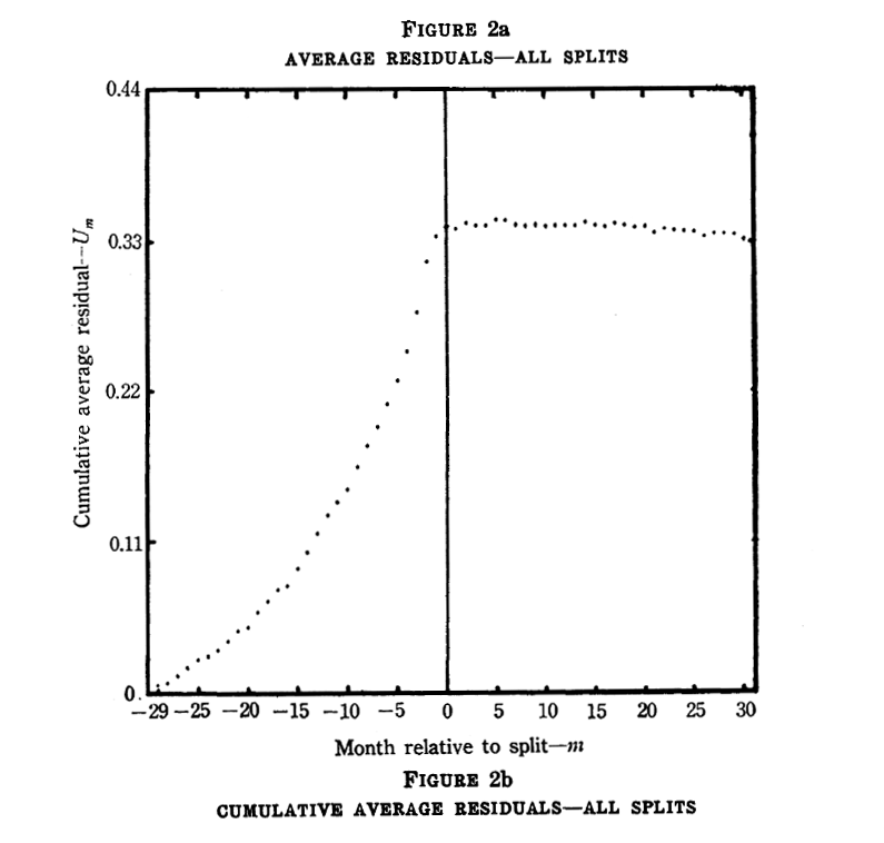
The actual chart from the 1969 Fama, Fisher, Jensen and Roll paper: it shows that on average, the price of a stock slowly increases up to the day of a stock split, after which it stays even
An event study of stock splits was actually the centerpiece of a famous 1969 paper that invented the idea. The paper remains a highly influential pillar of the "Efficient Market Hypothesis" school.
The analysis I found at Mechanical Markets was the same idea, except conducted for a much higher-frequency window of +/- 100 seconds. It also featured a logarithmic x axis, which allowed for very detailed analysis around "time 0" (the first tick is at +/- 10μs) as well as the trend over longer time frames.
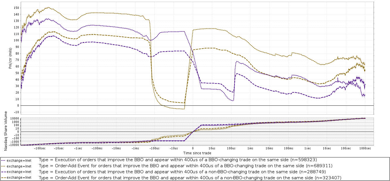
The high frequency event study I was trying to replicate, published by Mechanical Markets
I wanted to apply this type of analysis to my data. The first prototype I set out to build would use my own btc/usd trades as the study events, and measure the price changes across the whole market in the minutes before and after those trades.
Here's an example of the type high frequency event studies I ended up producing. This one shows the aggregate trend at several exchanges relative to each time a statistical "signal" fired (i.e. was present):
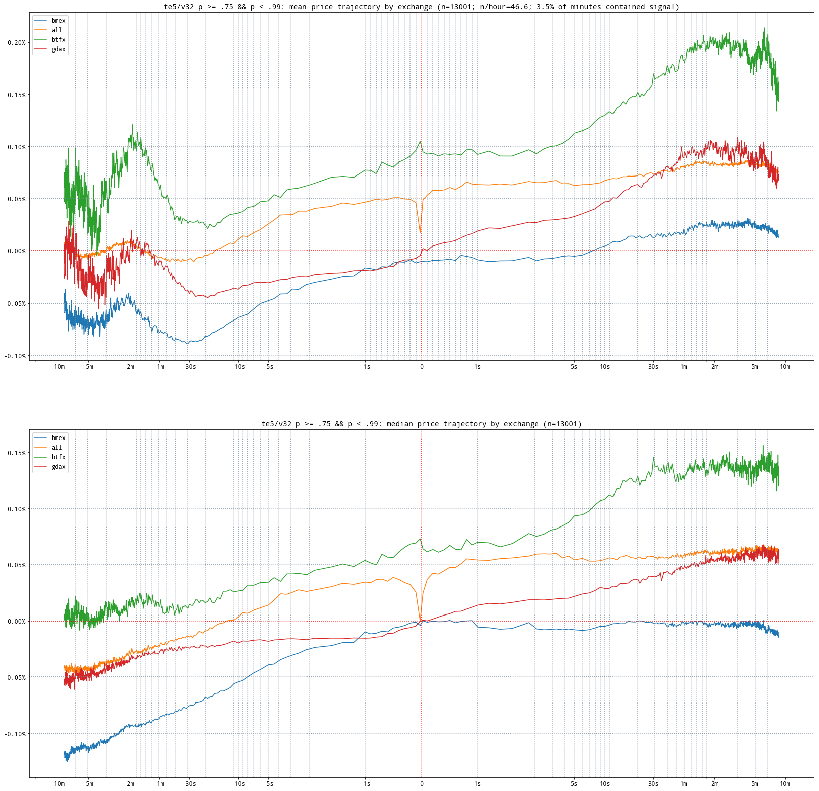
My take on high frequency event studies, produced some months after the day I wrote the first Rust prototype. You may notice the first tick comes at 1sec, instead of 10μs - crypto markets aren't there yet
What's So Hard About It?
When using Python libraries like Numpy for CPU-intensive numerical analysis, you want to write "vectorized" code as much as possible. Vectorized, in this sense, means code that utilizes Numpy-style array broadcasting (in systems programming, somewhat confusingly, the same term often refers to something else: whether a program's generated machine code utilizes SIMD instructions).
For instance, in zs = xs + ys, where xs and ys are arrays of the same shape using a library like Numpy, zs is assigned the elementwise addition of xs and ys.
The "vectorized" xs + ys is much faster than the equivalent Python list comprehension [xs[i] + ys[i] for i in range(len(xs))]. For two arrays of length 16,384, the list comprehension (13ms) is approximately 750x slower than the vectorized code (17μs).
There are two main reasons for such a dramatic performance difference:
- the C or Fortran code Numpy is using under the hood is highly optimized
- operating on the entire array in one statement (
xs + ys) greatly reduces the context switching between Python and C/Fortran code, which has its own overhead distinct from the cost of performing the actual calculations
Now, if you think about what calculations are involved in performing an event study-type analysis, you might start to see why it is not a good match for fast Python performance with Numpy and Pandas. For each event, you need to perform calculations relative to the event. That means many trips back-and-forth between the fast C code and the sloooowwwww Python code.
To put it another way: to maximize throughput, what you want is each operation to be on the entire length of the data you have. What an event study requires is many operations on small sections of the data.
The Python Implementation
That June day, I spent more time in Python than I did in Rust. I tried a lot of different tricks. I was working in a Jupyter notebook, using %time and %timeit to get microbenchmarks for all kinds of things.
My trades were in a Pandas DataFrame with 4,369,412 rows -- the global event set. I was performing the analysis on 1,100 of my trades (the study event set).
For each event, I was calculating the volume-weighted average price in 40 time buckets relative to the event time.
The final Python implementation I wrote is below, unaltered from the original, which I found preserved in a Jupyter notebook. Fair warning, it's ugly:
import numpy as np
import pandas as pd

def to_tframe(version, df, trades, start):
    d = {'bid': {}, 'ask': {}}
    cursor = 0
    n = 0
    n_periods = 40
    xs = np.concatenate([periods(n_periods)[:0:-1] * -1, periods(n_periods)]) * 1000000 # mult to convert to nanos
    mask = df['version'] == version
    my_trades = sorted(list(zip(df.loc[mask].index.values.astype(np.int64), df.loc[mask, 'side'], df.loc[mask, 'gid'])))
    idx = trades.index.values.astype(np.int64)
    amts = trades['amount']
    totals = trades['total']
    assert len(idx) == len(amts)
    assert len(idx) == len(totals)
    for tm, side, gid in my_trades:
        print '{} to_tfame {} {} (cursor = {})'.format(time.time() - start, version, n, cursor)
        min_time = tm + xs[0]
        max_time = tm + xs[1]
        if idx[cursor] > min_time:
            print 'warning: idx[cursor] ({}) > min_time ({})'.format(idx[cursor], min_time)
            while idx[cursor] > min_time and cursor > 0:
                cursor -= 1
        else:
            while idx[cursor] < min_time and cursor < len(idx) - 1:
                cursor += 1
        i = 1
        j = cursor
        d[side][gid] = {}
        while i < len(xs) - 1:
            wsum = 0.0
            w = 0.0
            while idx[j] < max_time:
                wsum += totals[j]
                w += amts[j]
                j += 1
            if w > 0.0:
                d[side][gid][xs[i]] = wsum / w
            else:
                d[side][gid][xs[i]] = np.nan
            i += 1
            min_time = max_time
            max_time = tm + xs[i]
        n += 1
    d['bid'] = sort_cols(pd.DataFrame.from_dict(d['bid'], orient='index'))
    d['ask'] = sort_cols(pd.DataFrame.from_dict(d['ask'], orient='index'))
    return d
If you know Python, you may notice this isn't a very "vectorized" implementation. All I can say is, I have distinct memories of attempting several vectorized approaches prior to this one.
Undoubtedly, there are faster ways to do this. Undoubtedly, there are cleaner, more maintainable ways to do this. All I'm claiming about that ambiguously-named, inscrutably implemented function to_tframe is, it's the fastest thing I could come up with June 9, 2018, and that I was, at that time, highly experienced at getting Python numeric code to run fast.
But, to_tframe wasn't fast -- it was glacial. At some point, I realized it was going to be far too slow to iterate on, so I just set it up to keep running and switched tracks.
Later, I went back to check the damage. Here's what I found at end of the output:
4083.80027103 to_tfame 0.3.72-rc.7 1095 (cursor = 1236447)
4084.54927397 to_tfame 0.3.72-rc.7 1096 (cursor = 1236482)
4085.27251816 to_tfame 0.3.72-rc.7 1097 (cursor = 1236487)
4085.98719311 to_tfame 0.3.72-rc.7 1098 (cursor = 1236517)
4086.77543807 to_tfame 0.3.72-rc.7 1099 (cursor = 1236522)
4087.52675414 to_tfame 0.3.72-rc.7 1100 (cursor = 1236528)
4089.26303911 finished
4,089 seconds (or 68min, 9sec) later, it was finally done.
The Rust Implementation
I started a new binary called time-explorer to perform the analysis. My plan was to do the heavy lifting in Rust, then write the aggregations out to CSV, which I could analyze further in Python.
The first task was parsing trades data from a CSV file I was using.
Thanks to the wonderful Serde and CSV crates, that part was a cinch. First I defined a Trade struct that derived Deserialize:
#[derive(Deserialize)]
struct Trade {
    pub time: i64,
    pub price: f64,
    pub amount: f64,
}
Since for this analysis I only cared about those three fields (time, price, and amount), I just left the other columns out, and they were ignored.
If you don't know Serde, what a #[derive(Serialize, Deserialize)] attribute gets you is fast, automatic serialization and deserialization in 16 different formats.
JSON:
let json = r#"{"time":1527811201900505632,"price":7492.279785,"amount":0.048495,"exch":"bits","server_time":0,"side":null}"#;

serde_json::from_str::<Trade>(json) // -> Ok(Trade { time: 1527811201900505632, price: 7492.279785, amount: 0.048495 })
CSV:
let csv = "time,amount,exch,price,server_time,side\n\
           1527811201900505632,0.048495,bits,7492.279785,0,";

let mut csv_reader = csv::Reader::from_reader(csv.as_bytes());

let headers = csv_reader
    .headers()
    .expect("parsing row headers failed")
    .clone();

let mut row = csv::StringRecord::new();

csv_reader.read_record(&mut row);           // -> Ok(true)

row.deserialize::<Trade>(Some(&headers));   // -> Ok(Trade { time: 1527811201900505632, price: 7492.279785, amount: 0.048495 })
Other supported formats include YAML, TOML, x-www-form-urlencoded, MessagePack, BSON, Pickle, CBOR, Bincode, and others. Serde is fantastic, and an awesome part of using Rust.
The CSV crate can parse full rows into structs implementing Deserialize (like Trade), so the parsing code went like this:
let mut trades: Vec<Trade> =
    csv::Reader::from_reader(trades_csv)
        .deserialize()
        .map(|x| x.unwrap())
        .collect();
In a production system, calling .map(|x| x.unwrap()) on each row would be extremely unwise. If one row failed to parse, it would crash the program. In a short-running data munging script, it's not a big deal.
Similarly, in a program like this I generally pepper the whole program with assert! statements to verify the integrity of the data, especially things like array lengths that aren't (currently) encoded in the type system. In this situation, silent data corruption is far worse than a crash.
Once the CSV file was parsed, I sorted the data by time and switched its memory layout from rows to columns, so to speak:
trades.sort_by_key(|k| k.time);

let mut times: Vec<i64> = Vec::with_capacity(trades.len());
let mut amounts: Vec<f64> = Vec::with_capacity(trades.len());
let mut totals: Vec<f64> = Vec::with_capacity(trades.len());

for Trade { time, price, amount } in trades {
    times.push(time);
    totals.push(price * amount);
    amounts.push(amount);
}
Notice that instead of storing a prices vec, I have a totals vec instead. The motivation for this is, to compute the weighted average inside each time bucket, I will be calculating
sum(p * a for p, a in zip(prices[i:j], amounts[i:j])) / sum(amounts[i:j])
... for some range of trades rows i..j. By storing totals rather than prices, I can instead compute the
sum(totals[i:j]) / sum(amounts[i:j])
... potentially saving many multiplications, as the prices[i] * amounts[i] multiplication is only done once per row, and I am likely to hit the same rows many times over the course of the analysis.
I also parsed a separate file with the timestamps for my study events into an Event struct:
#[derive(Deserialize)]
struct Event {
    pub time: i64,
    pub data: Vec<f64>, // holds the computed values for each time bucket for this study event
}
With the study events parsed, it's time do some event studying.
The Hard Part
The nested loops I came up with to do the analysis are admittedly a bit gnarly (it's a relatively faithful port of to_tframe actually):
let mut cursor: usize = 0; // current position in `times`/`totals`/`amounts` vecs

let n: usize =             // [..] number of time buckets. set by cli option.

let buckets: Vec<i64> =    // [..] the time buckets to compute the weighted average for, in
                           //      nanoseconds delta from study event time. buckets[0] is a
                           //      negative value, so the range buckets[0]..buckets[1] is
                           //      a period before the study event occurs (and the earliest bucket).
                           //      the range buckets[buckets.len()-2]..buckets[buckets.len()-1]
                           //      is two positive values, and the furthest bucket into the future
                           //      relative to the study event.

'a: for (i, event) in events.iter_mut().enumerate() {

    let mut min_time: i64 = event.time + buckets[0]; // current "left edge" of time bucket we are computing for
    let mut max_time: i64 = event.time + buckets[1]; // current "right edge" of time bucket we are computing for

    'b: while times[cursor] > min_time && cursor > 0 { cursor -= 1; } // see note below for details

    // find the start of this event's time buckets
    'c: while times[cursor] < min_time {
        if cursor >= times.len() - 1 { break 'a }
        cursor += 1;
    }

    let mut j: usize = cursor;

    'd: for k in 0..(n - 2) {

        let mut wsum: f64 = 0.0; // will store sum(  totals[cursor..j] ) where cursor,j are index bounds of this time bucket
        let mut w   : f64 = 0.0; // will store sum( amounts[cursor..j] ) where cursor,j are index bounds of this time bucket

        'e: while j < times.len() - 1 && times[j] < max_time {
            wsum +=  totals[j];
            w    += amounts[j];
            j    += 1;
        }

        // store weighted average for this time bucket
        event.data[k] = if w > 0.0 { wsum / w } else { std::f64::NAN };

        // increment time bucket
        min_time = max_time;
        max_time = event.time + buckets[k + 2];
    }
}
This implementation relies on both the trades arrays and the study events array being sorted. Since they are sorted, the next study event will always be past the last one. The bounds of the time buckets are computed relative to the study event's time, and will be nearby (and likely in the CPU cache) from the spot the loop has iterated to.
The hardest part of writing this code was the off-by-one errors from all the delicate indexing operations. It took some effort to get right. It's very easy to get confused when you have one array (buckets) that represents the edges of the values in another array, and then you need to find the indices in the second array corresponding to slots with values that are adjacent to the bucket edge values in the first array (phew!).
Nowadays, the unused loop labels (i.e. 'b, 'c, 'd, e) get an unused_labels warning from rustc -- they didn't when I wrote this. Personally, they help me think about the structure of some very dense, nested loops, whether or not the code actually uses them. Maybe that's just me.
While cleaning this up, I spotted a bug. The line 'b: while times[cursor] > min_time && cursor > 0 { cursor -= 1; } wasn't in the original. Without it, it's possible for the previous loop iteration to advance past the earliest time buckets for the next event (i.e. if times[cursor] > min_time at the top of loop 'a. The way the code is designed, the consequences of this are potentially incomplete analysis for some time buckets if two study events are close enough together, or, if cursor had also advanced past max_time, buckets skipped altogether. I added some counters to the loop to diagnose the impact: using a larger data set than when I built the first time-explorer, the bug resulted in 215 skipped time buckets and 730 incomplete data time buckets, out of a total of 899,856 total time buckets. While the impact was quite limited, it's a good reminder to stay sharp.
After completing the analysis, the program writes the output to a CSV file, which is pretty routine. But, the final thing I added was a CLI menu built with the Clap crate:
let args: clap::ArgMatches = clap::App::new("time-explorer")
    .version("0.1")
    .arg(clap::Arg::with_name("trades")
         .long("trades-csv")
         .short("t")
         .help("Path of csv with time (integer nanoseconds timestamp), \
                price (f64), and amount (f64) columns.")
         .takes_value(true)
         .required(true))
    .arg(clap::Arg::with_name("events")
         .long("events-csv")
         .short("e")
         .help("Path of csv file with a time (integer nanoseconds timestamp) as column 0, \
                along with any other metadata columns that will be included in results")
         .takes_value(true)
         .required(true))
    .arg(clap::Arg::with_name("output")
         .long("output-file")
         .short("o")
         .help("Path to save results csv to")
         .takes_value(true)
         .required(true))
    .arg(clap::Arg::with_name("verbose")
         .long("verbose")
         .short("v"))
    .arg(clap::Arg::with_name("n-periods")
         .long("n-periods")
         .short("n")
         .help("Controls how many time buckets are evaluated")
         .takes_value(true)
         .default_value("50"))
    .get_matches();
The --help output:
time-explorer 0.1

USAGE:
    time-explorer [FLAGS] [OPTIONS] --events-csv <events> --output-file <output> --trades-csv <trades>

FLAGS:
    -h, --help       Prints help information
    -V, --version    Prints version information
    -v, --verbose

OPTIONS:
    -e, --events-csv <events>      Path of csv file with a time (integer nanoseconds timestamp) as column 0, along with
                                   any other metadata columns that will be included in results
    -n, --n-periods <n-periods>    Controls how many time buckets are evaluated [default: 50]
    -o, --output-file <output>     Path to save results csv to
    -t, --trades-csv <trades>      Path of csv with time (integer nanoseconds timestamp), price (f64), and amount (f64)
                                   columns.
Pretty nice! I love how easy that is.
When I ran this analysis for the first time in June 2018, the global trades CSV file had 4,369,412 rows and there were 1,100 events in the study set.
I was only able to find files with larger data sets for both: a trades CSV with 11,836,155 rows (2.7x the original data) and an events CSV with 18,747 rows (17x the original data).
But when I fired up time-explorer v0.1, execution time was still less than one second:
./target/release/time-explorer -t ../var/time-explorer/btc-usd/trades.csv -e ../var/time-explorer/btc-usd/my_trades.csv -o var/teout.csv --verbose
#    0.00s reading...
#    6.32s calculating...
#    6.32s     No.     0          NaN,      7637.32,      7643.62 ...
#    6.33s     No.   512      7701.29,      7706.13,      7708.57 ...
#    6.34s     No.  1024      7498.03,      7488.73,      7492.05 ...
#    6.35s     No.  1536      7438.60,      7452.81,      7433.43 ...
#    6.36s     No.  2048      7632.81,      7604.25,      7598.79 ...
#    6.37s     No.  2560      7608.89,      7624.22,      7628.91 ...
#    6.38s     No.  3072      7654.30,      7652.55,      7655.41 ...
#    6.39s     No.  3584      7720.13,      7723.60,      7715.98 ...
#    6.39s     No.  4096      7694.29,      7695.07,      7693.11 ...
#    6.40s     No.  4608      7663.73,      7657.47,      7656.74 ...
#    6.41s     No.  5120      7681.48,      7675.49,      7673.05 ...
#    6.42s     No.  5632      7568.57,      7557.18,      7571.07 ...
#    6.43s     No.  6144      7644.18,      7645.71,      7649.90 ...
#    6.43s     No.  6656      7645.69,      7646.39,      7653.64 ...
#    6.44s     No.  7168      7652.45,      7655.90,      7646.96 ...
#    6.45s     No.  7680      7664.94,      7671.65,      7669.66 ...
#    6.45s     No.  8192      7614.52,      7611.79,      7626.52 ...
#    6.47s     No.  8704      7297.09,      7310.70,      7310.43 ...
#    6.48s     No.  9216      7235.21,      7241.13,      7239.70 ...
#    6.51s     No.  9728      6830.22,      6818.21,      6857.73 ...
#    6.52s     No. 10240      6732.01,      6724.39,      6699.79 ...
#    6.53s     No. 10752      6536.09,      6517.65,      6425.04 ...
#    6.55s     No. 11264      6450.31,      6445.63,      6443.42 ...
#    6.58s     No. 11776      6366.25,      6410.68,      6559.79 ...
#    6.60s     No. 12288      6473.03,      6463.63,      6443.70 ...
#    6.61s     No. 12800      6500.16,      6498.74,      6510.93 ...
#    6.62s     No. 13312      6408.23,      6413.47,      6428.04 ...
#    6.64s     No. 13824      6706.12,      6720.87,      6732.83 ...
#    6.65s     No. 14336      6714.93,      6723.90,      6720.23 ...
#    6.66s     No. 14848      6745.45,      6743.03,      6744.32 ...
#    6.68s     No. 15360      5883.81,      5893.97,      5874.75 ...
#    6.69s     No. 15872      5930.25,      5885.04,      5835.80 ...
#    6.70s     No. 16384      6165.85,      6159.55,      6147.91 ...
#    6.71s     No. 16896      6279.92,      6290.18,      6306.97 ...
#    6.72s     No. 17408      6134.21,      6063.72,      6058.22 ...
#    6.73s     No. 17920      6068.31,      6080.82,      6082.38 ...
#    6.75s     No. 18432      6593.90,      6602.86,      6584.98 ...
#    6.76 writing... (n_time_buckets=899856, n_incomplete_buckets=0, n_skipped_buckets=0)
#    7.05 finished.
At 6.32sec it was "calculating" and at 6.76sec it was "writing" -- that leaves 0.44sec spent performing the event study analysis.
4089.26 / 0.44 # -> 9293.78

# python / rust = 9,294x slower!
Guido, call your office!
Conclusion
Was it worth it? This kind of analysis wasn't a run-once thing -- it was something I would iterate on heavily and go on to run hundreds of times in the following months, eventually on much, much larger data sets (hundreds of millions of rows). None of that would have been possible in Python. It just wouldn't have.
Another point is, this wasn't a case of going to the ends of the earth to eek out a tiny bit more performance. This was code I wrote in one sitting, in one afternoon, with a little over one year's experience writing Rust under my belt. And the first pass was just shockingly fast, compared to my expectations.
Finally, forget speed for a second -- which of these programs would you rather grok if you had zero familiarity with either one? As someone who just returned to this code long after I had forgotten all pertinent details, I can tell you it wasn't a difficult choice. The Rust code is far, far easier to follow given its static types, precise scoping rules, and overall explicitness. In contrast, diving into to_tframe to make changes sounds like a major headache to me, and I wrote it!
For me, this was an eye-opening experience. I knew it would be faster, but not that much faster. The amount of math a modern CPU is capable of if it's not sitting there, twiddling its thumbs waiting on memory to arrive is pretty astonishing. It also cemented my view that there were times and places in exploratory data analysis work where Rust could be an extremely valuable tool.
The Python code in the Jupyter notebook had already parsed the CSV, so I don't count the parsing time in my "less than one second" claim. For the record, Pandas reads the same file in around 10sec. With 10 minutes work (knowing what I know today), I was able to get CSV parsing down to 3.64sec, which brought the total runtime down to 4.38sec.
Notes and Further Reading
- I posted briefly about this at r/rust shortly after it happened
- Unadulterated, original
time-explorercode is here. Cleaned up version used while writing this article is here. - Original Python
to_tframeis here, and log output here (for the people in the r/rust comments who suggested I was making this all up)